Why Your Inbox Falls Behind: The Queueing Science of Email Overload

An inbox can become painfully slow before its owner runs out of time on an average day. The missing ingredient is variability: requests do not arrive evenly, difficult messages take longer than easy ones, and spare capacity is what absorbs those differences. When almost every available minute is already committed, a small disruption has nowhere to go except into tomorrow’s backlog.

That explanation changes the management question. Instead of asking why someone cannot keep their inbox empty, ask whether the work entering the system is compatible with the time available to complete it. A cleaner interface may remove friction. It cannot make an overloaded queue mathematically sustainable.

This feature develops an email-capacity model, explains where it applies, and provides a measurement protocol for a real workplace. The central result is deliberately conditional: in a simple queue with variable service times, increasing utilization from 80% to 90% can more than double average waiting time even though incoming work rises by only 12.5%. That is a model result, not a measurement of office workers or InboxCabin customers.

Research and commercial disclosure: This is an InboxCabin editorial research synthesis with original, reproducible calculations. It is not a new field experiment, a systematic review, or an independently peer-reviewed study. No cited study evaluated InboxCabin. All hypothetical inputs and modeled outcomes are labeled.

Ready for a simpler way to manage your email?

Try InboxCabin free for 30 days. No credit card required.

Start Free Trial

The evidence: what research establishes—and what it does not

John D. C. Little’s 1961 paper established the relationship now called Little’s Law: under its long-run conditions, average work in a system equals throughput multiplied by average time in the system. It connects backlog and delay; it does not identify why the backlog exists or guarantee that a short observation period is representative. 1

A separate 2015 email study examined more than two million Yahoo users and 16 billion messages in its broader dataset. As incoming load increased, the fraction of messages answered decreased even when replies became faster. Its observational, provider-specific data do not establish a universal email limit, but they warn against interpreting fast replies as proof that all work is being handled. 2

Queueing theory supplies the mathematical mechanism. The model used below is the M/G/1 queue: Poisson arrivals, one continuously available processor, independent handling durations, and first-come-first-served processing. Its average waiting-time relationship depends on utilization and variation in handling duration. It is a useful stress test, not a faithful description of every inbox. 3

Together, these sources justify a careful proposition: backlog deserves an operational explanation. They do not justify claiming that every worker loses a particular number of hours to email, that everyone should process messages continuously, or that one software purchase produces a specified gain.

Start with work items, not unread messages

Suppose a coordinator receives 120 messages. Fifty are automated updates requiring no action, thirty belong to existing conversations, twenty contain straightforward questions, and twenty introduce new work. Counting all 120 as equivalent demand would tell you very little about capacity.

Define an actionable work item instead. It might be an invoice that needs approval, a customer question that needs a substantive answer, or a scheduling request that must be resolved. A thread can contain several work items; several threads can concern the same one. Choose a counting convention before collecting data, and keep it consistent.

Reading is still work. The messages that require no answer may need screening, and that screening consumes time. The simplest first audit separates triage time from action time. Measure how much time is available for completing requests after triage and other responsibilities have been accounted for. Alternatively, model triage as its own stage. Do not count the same minutes in both stages.

Also separate waiting for someone else from waiting for your own attention. An invoice awaiting a supplier’s correction is not the same as an invoice nobody has opened. Both affect elapsed resolution time, but only one can be fixed by giving the coordinator another processing block.

A workable register therefore has four states: awaiting triage, ready for action, waiting externally, and completed. An unread badge has none of this information. It is an interface signal, not a capacity measure.

Calculate offered load before debating productivity habits

For a first approximation, define three quantities:

• Arrival rate: actionable requests entering the chosen workflow per hour.
• Average handling time: hands-on minutes required per request, including necessary checking and recording.
• Available processing time: time genuinely allocated to that workflow, excluding other duties and planned breaks.

Offered load is incoming work divided by available processing capacity. In the continuous model, utilization is ρ = λ × s, where λ is requests per minute and s is average handling time in minutes. In a daily planning worksheet, the analogous ratio is incoming requests multiplied by handling minutes, divided by available processing minutes.

Here is an explicitly hypothetical daily example. Ninety actionable requests at three minutes each require 270 minutes of work. If 300 minutes are available after meetings, triage, and other duties, the offered load is 90%. The employee has thirty minutes of spare processing capacity, not an entire spare day.

The arithmetic should include real work rather than only typing. If validating an answer takes two minutes and composing it takes one, a tool that halves composition time reduces the complete three-minute task to two and a half minutes. It does not halve the whole task. Likewise, moving a message to a folder does not complete the request contained in it.

This worksheet is already useful without sophisticated mathematics. A sustained ratio above 100% means demand exceeds the defined capacity. The possible responses are to reduce demand, reduce necessary handling time without sacrificing quality, add capacity, change the service promise, or consciously defer some work. Better personal discipline cannot eliminate that accounting identity.

Why 90% busy is very different from 80% busy

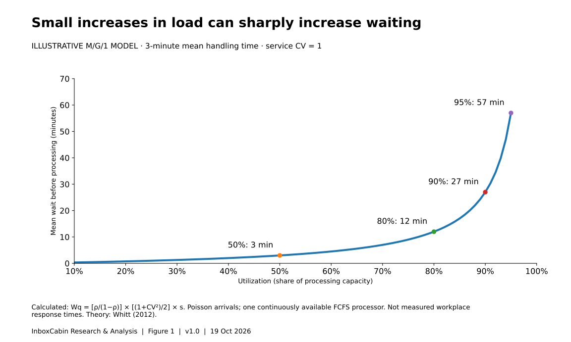
For the M/G/1 model, average waiting time before processing is:

Wq = [ρ ÷ (1 − ρ)] × [(1 + CV²) ÷ 2] × s

Here, CV is the standard deviation of handling time divided by its mean. Total time in the system is W = Wq + s. These are long-run means under the stated assumptions. The formula follows the Pollaczek–Khinchine relationship expressed in terms of handling-time variability. 3

To isolate the utilization effect, assume average handling time is three minutes and CV equals one. The variability factor then equals one. At 50% utilization, average waiting is three minutes. At 80%, it is twelve. At 90%, it is twenty-seven. At 95%, it is fifty-seven.

Download data (CSV)Download chart (SVG)View full-size chart

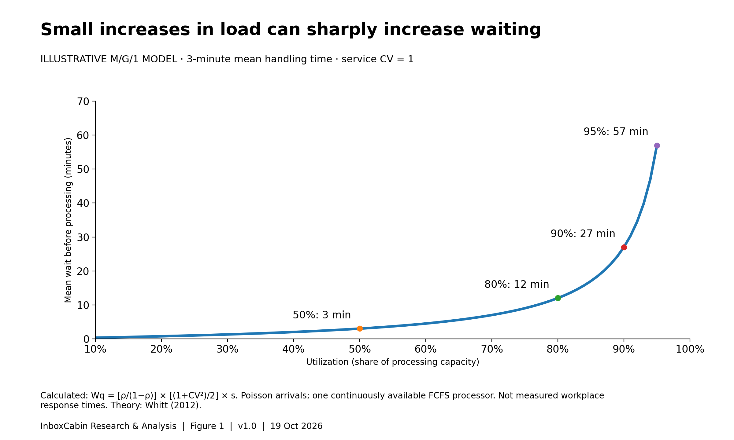
Read the chart data as a table

utilization percent	waiting minutes
50	3
80	12
90	27
95	57

Selected display values. Download the CSV for all rows and full precision; see caption for evidence type and units.

The jump from 80% to 90% utilization is only a 12.5% increase in arrival rate when handling time stays fixed. Yet modeled waiting rises from twelve to twenty-seven minutes: a 125% increase. This illustrates how an inbox could feel disproportionately worse after a modest increase in activity, without proving that the same numerical change occurs in an actual office.

Do not convert those minutes directly into a promise about business-hour response times. Real employees stop for meetings, work across channels, prioritize urgent items, and leave at the end of the day. The chart removes those features to show one mechanism. It is a warning about sensitivity near capacity, not a forecast for a particular employee.

Difficult requests change the equation even when averages look identical

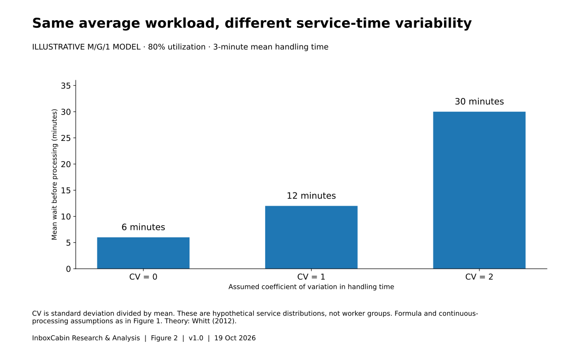
Consider three hypothetical workflows with the same three-minute mean handling time. In the first, every request takes three minutes. In the second, durations vary moderately. In the third, most requests are easy but a few require lengthy investigation.

At 80% utilization, the model produces six minutes of average waiting with CV zero, twelve minutes with CV one, and thirty minutes with CV two. Same average work per request. Same arrival rate. Different waiting because the variation differs.

Download data (CSV)Download chart (SVG)View full-size chart

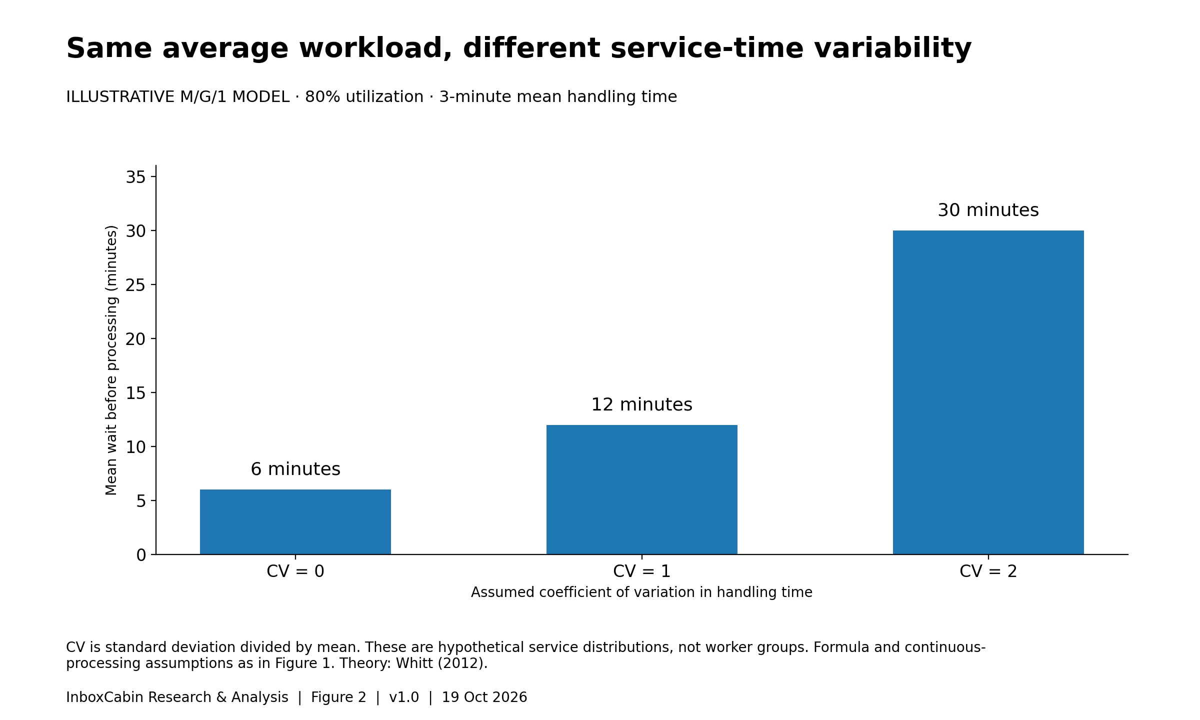
Read the chart data as a table

service cv	waiting minutes
0	6
1	12
2	30

Selected display values. Download the CSV for all rows and full precision; see caption for evidence type and units.

This suggests a practical investigation: which requests have unpredictable handling times, and why? Missing information, unclear authorization, uncertain ownership, or repeated exceptions might be contributing. The right intervention could be a better intake form or a clearer approval rule rather than a faster email application.

A separate lane for complex cases is sometimes useful, but it is not free capacity. Someone must still do that work. Separating queues can also strand capacity if one person is idle while another is overloaded. Evaluate the whole workflow, not just the lane whose numbers look better after the change.

Preserve fairness, too. If the easiest requests are always completed first, the overall average may improve while difficult customers wait indefinitely. Report the age and number of unresolved exceptions alongside average turnaround. A healthier average is not a success when it hides a deteriorating tail.

Spare capacity is also what clears yesterday’s backlog

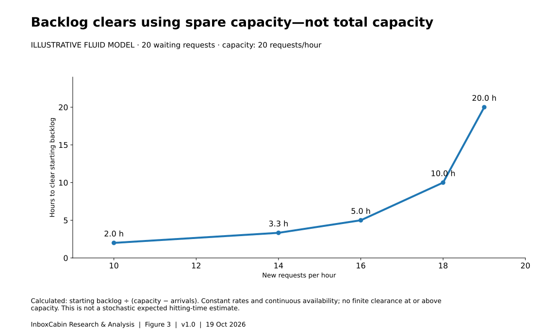
A second calculation makes the value of slack easier to see. Imagine a starting backlog of twenty requests, processing capacity of twenty requests per hour, and eighteen new requests arriving each hour. Only two requests per hour can be devoted to the old backlog. Under a simple fluid approximation, clearing those twenty requests takes ten hours—not one.

The equation is clearance time = starting backlog ÷ (capacity − arrival rate). It assumes constant rates, continuous availability, and no new interruptions. It is not a stochastic waiting-time formula.

With ten incoming requests per hour, the same backlog clears in two hours. With sixteen, it takes five hours. With nineteen, it takes twenty hours. If arrivals meet or exceed capacity, there is no finite clearance time for a positive starting backlog under these assumptions.

Download data (CSV)Download chart (SVG)View full-size chart

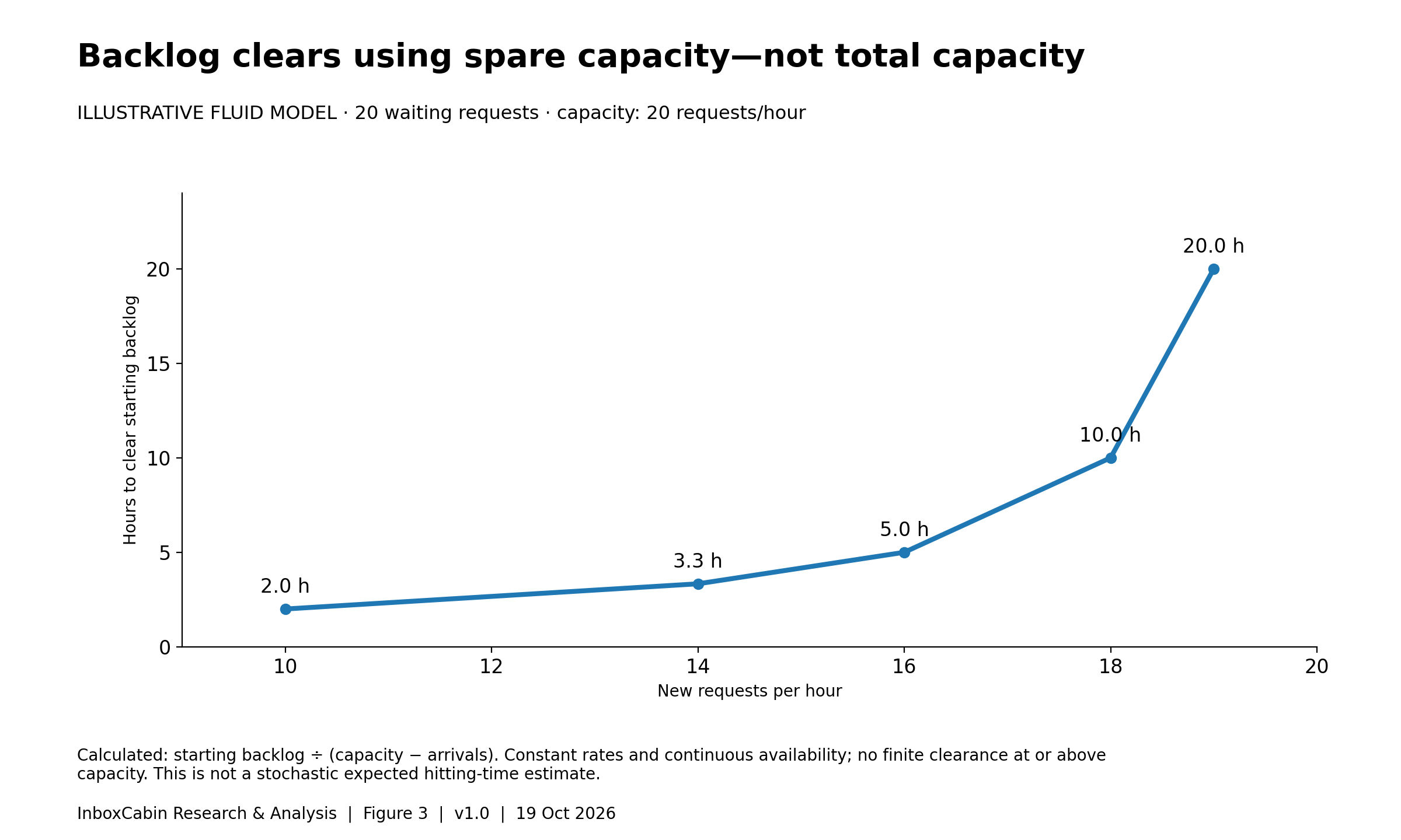
Read the chart data as a table

arrivals per hour	clearance hours
10	2
14	3.333
16	5
18	10
19	20

Selected display values. Download the CSV for all rows and full precision; see caption for evidence type and units.

This is why “just catch up this afternoon” can be an unrealistic instruction. The employee may have enough gross capacity to complete twenty requests, but most of that capacity is already committed to new arrivals. Catch-up requires net capacity.

A one-off overtime push can remove the starting backlog. It does not solve an ongoing imbalance. If the daily operating system recreates the backlog, treating each recurrence as a personal failure simply repeats an expensive cycle.

Use Little’s Law without turning it into a misleading dashboard

For a stable, consistently defined workflow, L = λW links average open work, throughput, and time in the system. If throughput is twenty completed requests per workday and average elapsed time is two workdays, the corresponding long-run average work in progress is forty requests. All three measures must use the same system boundary and compatible units. 1

That does not mean a snapshot of forty unread messages proves a two-day delay. A snapshot is not a time average; unread messages are not necessarily actionable requests; and the system may be growing rather than stable.

For measurement, count open actionable items at regular intervals across the day and average them. Record completions and arrival counts over the same period. Define whether the clock includes nights and weekends. Record items already open at the start and still open at the end. Otherwise, the hardest cases can disappear from turnaround statistics simply because they have not finished yet.

Track both the whole process and the actionable stage. A supplier delay may keep a case open for a week while consuming only six minutes of employee attention. That matters commercially, but it is not evidence that the employee needs seven days to write an email.

Finally, treat mismatches as diagnostic information. If the numbers do not approximately reconcile, inspect the definitions before blaming performance. Duplicate case counting, reopens, missing completions, and inconsistent business-hour clocks are plausible explanations worth checking.

An inbox can get faster while service gets worse

Suppose a team starts answering easy messages immediately and leaves difficult requests untouched. Median reply time may fall. The oldest unanswered requests may simultaneously become older. That would be a genuine improvement in one metric and a deterioration in another.

The Yahoo research provides a reason to look for this combination, not a license to assume it occurs everywhere. Its observed link between higher load and a lower reply fraction makes reply speed an incomplete indicator. The study was not a controlled test of service quality, and not every incoming message deserved an answer. 2

A balanced dashboard should therefore include completed work items, actionable backlog, age of the oldest unresolved items, reopens, and a small quality sample. Report counts next to percentages. Two missed requests out of ten and twenty missed out of one hundred have the same percentage but different operational consequences.

Do not rank employees by raw volume when their task mixes differ. Someone handling complicated payment disputes cannot be compared directly with someone acknowledging routine scheduling requests. A workload model is useful precisely because it makes these differences visible rather than hiding them inside an inbox count.

Where a dedicated email workspace can help

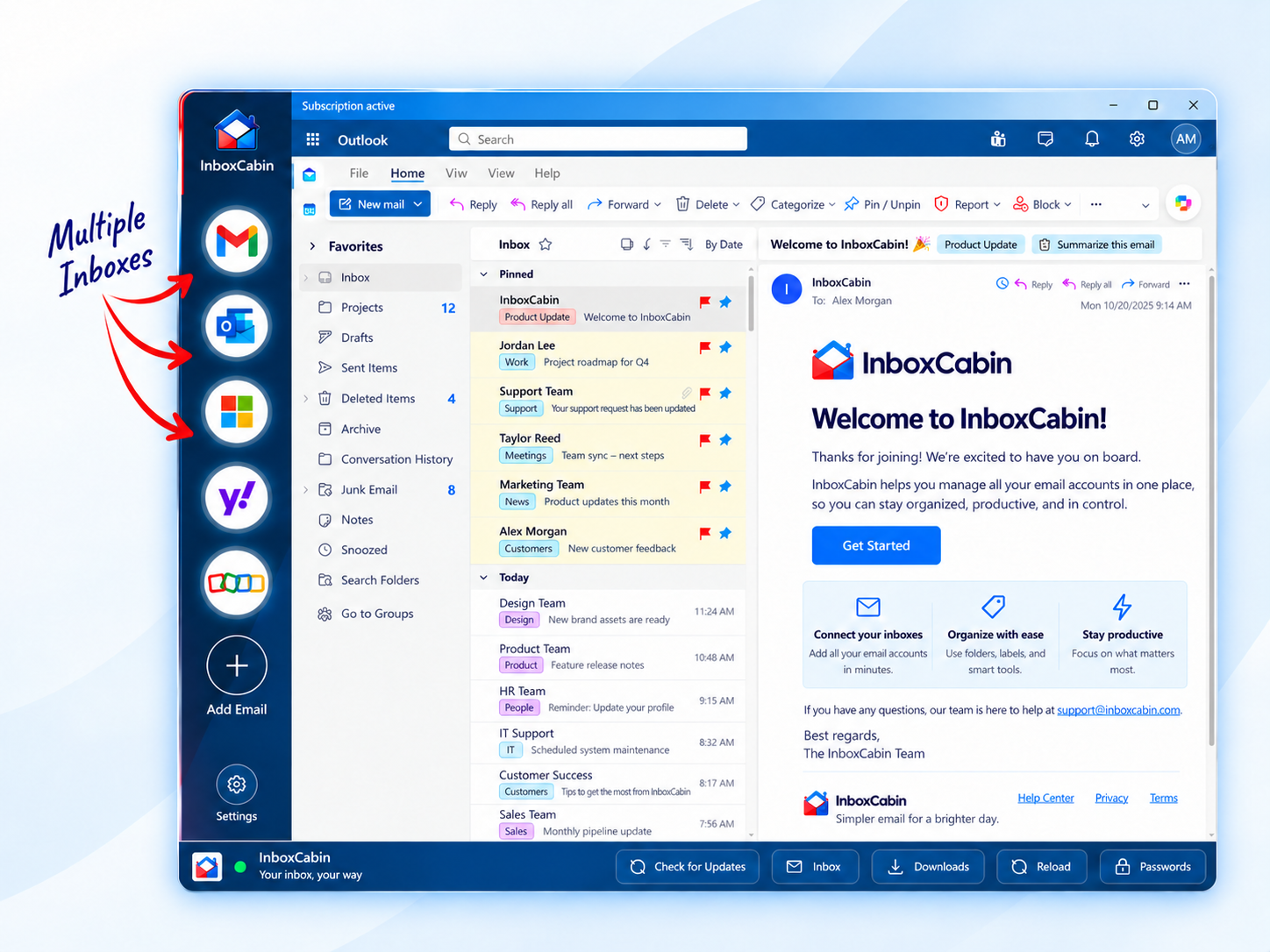
InboxCabin provides a dedicated Windows workspace for switching between separate Gmail and Microsoft inboxes. That can be relevant when staff spend effort locating the correct account or navigating between unrelated browser windows. It is a potential reduction in navigation friction, not a change to incoming demand or an automatic increase in staffing capacity.

The queue model should not be used as proof of an InboxCabin time saving. None of the cited studies tested the product. Measure the complete workflow with and without the workspace, including mistakes and rework. Provider sign-in requirements, employer policies, and the underlying email features still apply.

Download Now

30-day free trial · Bring your email accounts together in one Windows workspace.

A practical four-week capacity investigation

Week one: define the system. Select one repeatable workflow, such as incoming quote requests, rather than all company email. Agree on what counts as arrival, completion, external waiting, and a reopened case. Write down working hours and the promised service level. Do not collect private message text when counts and timestamps will answer the question.

Week two: establish a baseline. Measure several normal workdays, noting holidays, unusually large projects, and absences. Use a small voluntary sample of active handling durations, not an assumption that an open window means continuous work. Estimate both the mean and the spread. Keep an unusually difficult case from being silently deleted as an “outlier” if such cases genuinely recur.

Week three: change one plausible constraint. Options include improving intake completeness, assigning a clear owner, protecting a processing block, or reducing navigation between accounts. Document the intervention precisely. Do not simultaneously change staffing, triage policy, and software and then attribute the whole difference to the software.

Week four: compare outcomes and side effects. Evaluate actionable backlog, age distribution, completion rate, quality, and staff experience. Compare comparable workdays and task types. A short before-and-after pilot can suggest a useful direction, but seasonality, learning, and workload differences limit causal claims. A randomized or counterbalanced design is stronger when practical.

Publish the result internally even when the intervention does not help. Discovering that navigation was not the bottleneck can prevent further spending and redirect attention to approval delays or excessive intake. A useful experiment resolves uncertainty; it does not have to vindicate the original idea.

Three choices a manager can make with the model

Reduce unnecessary arrivals. Consider whether a form could answer a recurring question before it becomes a request, whether one digest could replace repeated updates, or whether the right person could receive the first message. These are design hypotheses. Test whether they reduce actual handling work rather than merely moving it to another channel.

Reduce necessary effort per completed request. Better context, reusable verified information, and clear decision authority may remove repeat work. A faster reply that creates another clarification round is not necessarily cheaper. Include the follow-up effort when judging the intervention.

Provide a realistic capacity margin. Capacity may come from backup coverage, workload balancing, or adjusting deadlines. The model does not establish a universal ideal utilization percentage. A predictable, low-consequence workflow can tolerate a different operating point from a volatile, time-sensitive one. Choose the margin against observed service performance and consequences, not a slogan about staying busy.

There is also a fourth choice: change the promise. Some requests genuinely do not require immediate attention. A truthful next-business-day commitment may be better than an informal expectation of instant replies that the system cannot sustain. Protect truly urgent requests with a separate escalation route and named coverage, not with the hope that everybody watches every inbox constantly.

Methods, assumptions, and how to reproduce the charts

The evidence selection was a targeted narrative review, checked on October 19, 2026. It includes an original queueing theorem, a queueing teaching reference, and an empirical email-behavior study. It is not an exhaustive literature search. No private inboxes were accessed and no customer performance data were collected for this article.

Figures 1 and 2 are exact calculations within the specified M/G/1 model, not simulations. Figure 3 uses a separate deterministic clearance equation. The accompanying CSV files and Python script contain the input values and calculations. Both approaches intentionally omit priorities, employee breaks, team handoffs, nonstationary demand, and external approval delays.

The most important sensitivity is what gets counted as service. A three-minute estimate that omits preparation or recording will understate load. Likewise, a calendar hour is not a processing hour if most of it is committed to meetings. Make those boundaries explicit before entering numbers into the calculator.

The downloadable worksheet leaves operational observations blank. Sample chart values are labeled illustrative. There are no fabricated confidence intervals: mathematical scenarios do not become empirical studies because they are drawn precisely. To cite the model, identify the assumptions along with the result and credit the original queueing sources separately.

The conclusion: stop measuring effort without measuring demand

An overwhelmed inbox can reflect an overwhelmed system. The most useful response is not automatically another notification rule, another reminder to work faster, or another app. It is a clear account of incoming work, handling effort, variability, and available capacity.

The practical lesson is modest but powerful: spare capacity is not necessarily waste; it is the mechanism that absorbs unpredictable work and clears backlogs. When a team understands that mechanism, it can make better choices about tools, staffing, intake, and service promises.

For people whose measurable friction is switching between Gmail and Microsoft accounts, InboxCabin offers a focused desktop workspace. Evaluate it against that specific problem. Keep the capacity model honest enough to show when the actual constraint lies somewhere else.